Plus 2.X:First Steps: Unterschied zwischen den Versionen
Krizzl (Diskussion | Beiträge) |
SebSta (Diskussion | Beiträge) |
||
| (19 dazwischenliegende Versionen von einem anderen Benutzer werden nicht angezeigt) | |||
| Zeile 1: | Zeile 1: | ||
'''Example Case | '''Example Case | ||
This short example | This short example shows you step by step how to input and calculate a case. To create and compute a new case, please perform the 13 following steps. There is also a [http://www.wufi-wiki.com/wufifilme/overview_movie/rohfassung.htm '''movie'''] demonstrating all the steps. | ||
''' | ''' | ||
== STEP one: Information and setting of | == STEP one: Information and setting of framework conditions == | ||
| Zeile 11: | Zeile 12: | ||
[[Bild:11_examplecase.png|1:Creating an example case|center|frame|Figure 1:Creating an Example Case]]<br> | [[Bild:11_examplecase.png|1:Creating an example case|center|frame|Figure 1:Creating an Example Case]]<br> | ||
== STEP two : Definition of the climatic | == STEP two : Definition of the climatic conditions == | ||
| Zeile 24: | Zeile 25: | ||
For advanced users: It is also possible to define own climate conditions or to [[Plus 2.X:Files/Measured Data|import own climate files]]. | For advanced users: It is also possible to define own climate conditions or to [[Plus 2.X:Files/Measured Data|import own climate files]]. | ||
As long as your building does not float in the air, for whatever reason, it is necessary to define at least one additional climate to give reasonable boundary conditions for the inert behavior of soil. This can be done using the “[[Plus 2.X:Dialog_Climate#Optional Climate|Optional Climates]]” tab. For the soil temperature it is accurate to select a sine curve that has its peak at about two months later than summer solstice, i.e. at the end of August / in early September in the northern hemisphere. Depending on local conditions, the amplitude of the sine curve can be modified due to the annual fluctuation of the temperature curves. This fluctuation is the difference of the mean maximum temperature of soil in warm seasons and the mean minimum temperature of soil in cold seasons. For continental climates like Siberia this amplitude may be high (high temperatures in summer, very cool winter), for maritime climate systems it is rather low. Furthermore, the mean temperature must be set. This can be approximated using the annual average air temperature. In this example we assume the climate of Holzkirchen, the | As long as your building does not float in the air, for whatever reason, it is necessary to define at least one additional climate to give reasonable boundary conditions for the inert behavior of soil. This can be done using the “[[Plus 2.X:Dialog_Climate#Optional Climate|Optional Climates]]” tab. For the soil temperature it is accurate to select a sine curve that has its peak at about two months later than summer solstice, i.e. at the end of August / in early September in the northern hemisphere. Depending on local conditions, the amplitude of the sine curve can be modified due to the annual fluctuation of the temperature curves. This fluctuation is the difference of the mean maximum temperature of soil in warm seasons and the mean minimum temperature of soil in cold seasons. For continental climates like Siberia this amplitude may be high (high temperatures in summer, very cool winter), for maritime climate systems it is rather low. Furthermore, the mean temperature must be set. This can be approximated using the annual average air temperature. In this example we assume the climate of Holzkirchen, the WUFI®’s origin with moderate continental climate. How this can be entered in WUFI®plus can be seen in Figure 4 on the next page. | ||
[[Bild:14_soilclimate.png|center|frame|Figure 4:Setting of an optional climate]]<br> | [[Bild:14_soilclimate.png|center|frame|Figure 4:Setting of an optional climate]]<br> | ||
| Zeile 40: | Zeile 41: | ||
For relative humidity a constant mean value of 99% is adequate. | For relative humidity a constant mean value of 99% is adequate. | ||
== STEP three: Generate | == STEP three: Generate building geometry == | ||
For generating the geometry, there are two basic options. Rather simple buildings or space can be created using the [[Plus 2.X:Building#Building Wizard|automatic building wizard]]. This tool generates a building with predefined floor plan, roof and foundation selections. Here we assume a simple case with one heated slab-on-ground zone and an inclined unheated attic. Figure 5 indicates the steps to generate a simple standalone building. There is also | For generating the geometry, there are two basic options. Rather simple buildings or space can be created using the [[Plus 2.X:Building#Building Wizard|automatic building wizard]]. This tool generates a building with predefined floor plan, roof and foundation selections. Here we assume a simple case with one heated slab-on-ground zone and an inclined unheated attic. Figure 5 indicates the steps to generate a simple standalone building. There is also the possibility of defining the orientation of the main facade of the building as highlighted at the bottom of in Figure 15. | ||
If, however, a more complex building is requested, it can be [[Plus 2.X:Building#Edit 3D|created using vertices]]. | If, however, a more complex building is requested, it can be [[Plus 2.X:Building#Edit 3D|created using vertices]]. | ||
| Zeile 70: | Zeile 71: | ||
Checking the Caption Bar of the “Component Openings” window defines whether the wall is viewed from inside or outside. | Checking the Caption Bar of the “Component Openings” window defines whether the wall is viewed from inside or outside. | ||
The new window will be shown under [[Plus 2.X:Visualized Components|Visualized Components]]. So the windows and openings | The new window will be shown under [[Plus 2.X:Visualized Components|Visualized Components]]. So the windows and openings will appear in the navigation tree and can be edited as usual. | ||
[[Bild:16_windows2.png|center|frame|Figure 6:Generating windows]]<br> | [[Bild:16_windows2.png|center|frame|Figure 6:Generating windows]]<br> | ||
| Zeile 76: | Zeile 77: | ||
For advanced users: It is also possible to generate openings by using the [[Plus 2.X:Building#Edit 3D|3D Edit tool]] or by defining own points. | For advanced users: It is also possible to generate openings by using the [[Plus 2.X:Building#Edit 3D|3D Edit tool]] or by defining own points. | ||
== STEP four: Definition of the | == STEP four: Definition of the components. == | ||
Primarily, a [[Plus 2.X:Visualized Components|component]] is a surface of the building. It may be the roof, the base plate or vertical walls. As the composition of our vertical walls is mostly the same, those can be summarized as one component. This is predefined in WUFI®Plus. | Primarily, a [[Plus 2.X:Visualized Components|component]] is a surface of the building. It may be the roof, the base plate or vertical walls. As the composition of our vertical walls is mostly the same, those can be summarized as one component. This is predefined in WUFI®Plus. | ||
To change this, click on the aimed component in the [[Plus 2.X:Visualization Box|Visualization Box]]. | To change this, click on the aimed component in the [[Plus 2.X:Visualization Box|Visualization Box]]. Afterwards, right click on this component, choose “Ungroup” and follow the instructions in accordance with your aimed modification. The “General” tab outlines basic data of a component and enables titling of components. This is especially important in case of numerous components for evaluating results. | ||
We start with Component 1 | We start with Component 1 the Bottom Plate according to the steps shown in Figure 7. Choose the component you want to edit in the Project Explorer [1], next assemblies can be allocated to a component in the “[[Plus 2.X:Visualized Components#Opaque components|Assembly]]” tab [2]. The Project construction list [3] shows all constructions used in a project. The highlighted one is applied to the respective component. As no constructions were assigned so far, the list is empty for one plain construction, which must be chosen. As there is no predefined geometry for the bottom plate, you have to define one, this is done by clicking the “Edit” button [4] which opens the “Edit Assembly” window [5] | ||
[[Bild:17_component12.png|center|frame|Figure 7:Editing an assembly]]<br> | [[Bild:17_component12.png|center|frame|Figure 7:Editing an assembly]]<br> | ||
| Zeile 136: | Zeile 137: | ||
Click [[Plus 2.X:Visualized Components#Opaque components|here]] for further information. | Click [[Plus 2.X:Visualized Components#Opaque components|here]] for further information. | ||
Assiging a [[Plus 2.X:Visualized Components#Transparent components|window]] type to the windows from the database works similar, please choose “Uncoated double glazing” for your window. | |||
Figure 11 illustrates the possibility of [[Plus 2.X:Visualized Components#Window Parameters|changing specific window parameters]]. The U parameter is the heat transfer coefficient. The frame factor enables description of opaque surfaces of the window. In effect, heat gains by solar radiation depend on the angle of incidence. In order to simulate this, the Solar Heat Gain Coefficient (SHGC) can be used. It can be set in general and with reference to the changing incident angle of solar radiation. There are appropriate predefined values, however they can be adjusted. The Emissivity of external surface is a value similar to the two previous items mentioned above. It expresses the amount of emitted radiation from the outer surface. | Figure 11 illustrates the possibility of [[Plus 2.X:Visualized Components#Window Parameters|changing specific window parameters]]. The U parameter is the heat transfer coefficient. The frame factor enables description of opaque surfaces of the window. In effect, heat gains by solar radiation depend on the angle of incidence. In order to simulate this, the Solar Heat Gain Coefficient (SHGC) can be used. It can be set in general and with reference to the changing incident angle of solar radiation. There are appropriate predefined values, however they can be adjusted. The Emissivity of external surface is a value similar to the two previous items mentioned above. It expresses the amount of emitted radiation from the outer surface. | ||
| Zeile 151: | Zeile 152: | ||
Also user defined assemblies can be saved in the database, this is reasonable, if you want to reuse assemblies as you don’t have to define them using the “Edit” button (like you did defining the bottom plate) each time but can easily select it from the database. | Also user defined assemblies can be saved in the database, this is reasonable, if you want to reuse assemblies as you don’t have to define them using the “Edit” button (like you did defining the bottom plate) each time but can easily select it from the database. | ||
Watch this [http://www.wufi-wiki.com/wufifilme/step6-components/Bottom_Plate_assemblydatabase/step6_Bottom_Plate.htm '''movie'''] to see how user defined assemblies can be saved to the database. | |||
== STEP five: Definition of | == STEP five: Definition of “not visualized components” == | ||
| Zeile 178: | Zeile 180: | ||
|}<br style="clear:both" /> | |}<br style="clear:both" /> | ||
== STEP six: Setting of | == STEP six: Setting of inner loads (occupancy schedule) == | ||
| Zeile 190: | Zeile 192: | ||
For advanced users: Another option for getting inner loads is to load an own schedule for supported file types using [[Plus 2.X:Files/Measured Data|Files/Measured Data.]] | For advanced users: Another option for getting inner loads is to load an own schedule for supported file types using [[Plus 2.X:Files/Measured Data|Files/Measured Data.]] | ||
== STEP seven : Defining | == STEP seven : Defining design inner climate conditions == | ||
Step seven is related to step six. In this step you have to verify the [[Plus 2.X:Design Conditions|design conditions]], i.e kind of heating/cooling and the ventilation system. Preliminary it is important to know that for indoor climate conditions two basic requirements are necessary: | Step seven is related to step six. In this step you have to verify the [[Plus 2.X:Design Conditions|design conditions]], i.e kind of heating/cooling and the ventilation system. Preliminary it is important to know that for indoor climate conditions two basic requirements are necessary: | ||
*a schedule to control working hours of heating, cooling, de-/humidification or ventilation system and | *a schedule to control working hours of heating, cooling, de-/humidification or ventilation system and | ||
*a definition of capacities of these systems. see [[#STEP eleven: Initiation of HVAC | *a definition of capacities of these systems. see [[#STEP eleven: Initiation of HVAC systems|STEP eleven: Initiation of HVAC Systems]] or [[PLus 2.X:HVAC|HVAC]] | ||
In this step, the schedules for our design conditions (the conditions to be maintained by the HVAC equipment) are defined. The indoor atmospheric conditions should conform to a certain range of temperature and relative humidity. Limits for those parameters can be set in this section. According to a healthy room temperature, in this example we use the following parameters: | In this step, the schedules for our design conditions (the conditions to be maintained by the HVAC equipment) are defined. The indoor atmospheric conditions should conform to a certain range of temperature and relative humidity. Limits for those parameters can be set in this section. According to a healthy room temperature, in this example we use the following parameters: | ||
| Zeile 239: | Zeile 241: | ||
It is also possible to input values for “Relative Humidity” and “Max. CO2 Concentration” | It is also possible to input values for “Relative Humidity” and “Max. CO2 Concentration” | ||
== STEP nine : Other | == STEP nine : Other parameters == | ||
The entries in | The entries in “[[Plus 2.X:Other Parameters|Other Parameters]]” remain unchanged in this example. The standard values in this entry are shown below. | ||
[[Bild:26_otherparameters.png|16:Other parameters]]<br> | [[Bild:26_otherparameters.png|center|frame|Figure 16:Other parameters]]<br> | ||
For advanced users: The modification of solar gains can be changed in this entry, as well. In terms, the factor of direct solar radiation to the inner air and the distribution of solar radiation on the inner surfaces can be altered. The “former factor” means the fraction of solar radiation that directly heats up the inner air; the higher the value, the more direct solar heating of inner air. The latter describes different energy gains by inner surfaces. This factor can be kept proportional to the surface areas or set user-defined. Further “Other Parameters” are initial conditions of temperature, CO2 concentration and relative humidity as well as an accuracy interval of the simulation. The lower the accuracy, the faster the calculation. | For advanced users: The modification of solar gains can be changed in this entry, as well. In terms, the factor of direct solar radiation to the inner air and the distribution of solar radiation on the inner surfaces can be altered. The “former factor” means the fraction of solar radiation that directly heats up the inner air; the higher the value, the more direct solar heating of inner air. The latter describes different energy gains by inner surfaces. This factor can be kept proportional to the surface areas or set user-defined. Further “Other Parameters” are initial conditions of temperature, CO2 concentration and relative humidity as well as an accuracy interval of the simulation. The lower the accuracy, the faster the calculation. | ||
== STEP eight: Description of attached zones == | |||
In this example, our [[Plus 2.X:Attached Zones|attached zone]] is the roof toss. It is not heated, cooled or mechanical ventilated but normally, it also differs from the outer climate. The menu item “Attached Zones” enables the user to assign optional climates to such areas of the building. Nevertheless, in our case the outer climate is taken as reference. Otherwise it would have been necessary to define an additional optional climate. | |||
[[Bild:27_attachedzones.png|center|frame|Figure 17:Definition of attached zones]]<br> | |||
== STEP ten: 3D Objects & remaining elements == | == STEP ten: 3D Objects & remaining elements == | ||
“3D objects” allows WUFI plus calculation of three dimensional thermal bridges under transient boundary conditions. In the folder “remaining Elements” surrounding of the building like trees etc. can be established | “3D objects” allows WUFI plus calculation of three dimensional thermal bridges under transient boundary conditions. In the folder “remaining Elements” surrounding of the building like trees etc. can be established. | ||
== STEP eleven: Initiation of HVAC systems == | |||
Like previously mentioned in step seven, it is important not only to schedule [[PLus 2.X:HVAC|HVAC systems]] but also to assign capacities to those facilities. First it is necessary to establish these three systems like shown in Figure 18 in the red boxes. These three systems are established by hitting the “New” button three times. The type of system is selected in the “Kind” field by clicking into the blank field of the new device whereas a drop-down menu opens that suggests different system types. These are heating, cooling, de-/humidification and mechanical ventilation facilities. | |||
[[Bild:28_HVAC1.png|center|frame|Figure 18:Establishment of HVAC]] <br> | |||
[ | In consequence, the entries marked in the green box will appear in the project explorer. Furthermore, the facilities need characteristic values for the capacities. Please be aware that all systems are ideal systems – which means the assigned capacity is available immediately and without heat losses. Following Figure 19, the capacity of the heating system is defined 40 [kW]. In this case a schedule for the capacities is renounced as fixed facilities which serve to maintain a certain room climate are assumed. This procedure is repeated in the example for the “Cooling System”, with a capacity of 40 [kW], as well. | ||
[[Bild:29_HVAC2.png|center|frame|Figure 19:Assigning capacities to HVAC systems (1)]]<br> | |||
[[ | In the [[Plus 2.X:Design Conditions|design conditions]], the air change due to mechanical ventilation is specified with 0,8 [1/h]. In order to meet this requirement, the necessary capacity of the ventilation system must be larger than 0,8*302.4 [m³/h], due to the room volume being 9*12*2.8 [m³]. So we could set 500 m³/h for the ventilation. Also a value for heat recovery from the ventilation system thus the efficiency of the ventilation system could be set. The whole input data is: | ||
{|border="1" align="left" style="text-align:center;" | |||
|Heating general | |Heating general | ||
|40kW | |40kW | ||
| Zeile 290: | Zeile 288: | ||
|60% | |60% | ||
|} | |} | ||
<br style="clear:both" /> | |||
This issue can be seen in the red box in Figure 20. The second red box in | This issue can be seen in the red box in Figure 20. The second red box in Figure 20 indicates the possibility of simulating a heat recovery system which is common for modern ventilation systems. A reasonable value for this is 60 [%]. | ||
[[Bild:30_HVAC3.png|center|frame|Figure 20:Assigning capacities to HVAC systems (2)]]<br> | |||
== STEP twelve: Simulation == | == STEP twelve: Simulation == | ||
If all the above mentioned data were entered, the Status/Results Box will show the “Start” simulation button. Pressing | If all the above mentioned data were entered, the [[Plus2:Status and Results|Status/Results Box]] will show the “Start” simulation button. Pressing it, hygrothermal calculation will start. If the “Start” button does not appear in the Status/Results Box and there is an error message, double-click on the error message and the program will automatically jump to the incorrect entry. | ||
[[Bild:31_startcalculation.png|21:Start calculation]]<br> | [[Bild:31_startcalculation.png|center|frame|Figure 21:Start calculation]]<br> | ||
During the computation process, the simulated temperature humidity distribution in the element can be observed in real time for all components. Figure 22 shows this for our side walls. The calculation can be accelerated by deactivating this option. This can be done by clicking on the “Maximum speed” button (green box in Figure 22). | During the computation process, the simulated temperature humidity distribution in the element can be observed in real time for all components. Figure 22 shows this for our side walls. The calculation can be accelerated by deactivating this option. This can be done by clicking on the “Maximum speed” button (green box in Figure 22). | ||
[[Bild:32_resultsduringcalc.png|22:Results during calculation]]<br> | [[Bild:32_resultsduringcalc.png|center|frame|Figure 22:Results during calculation]]<br> | ||
== STEP thirteen: Analysis of the | == STEP thirteen: Analysis of the results == | ||
The final results of the calculations can be looked at in several ways. First, the general results can be seen like depicted in Figure 24. The Excel export, or in general, the “Export to file” button are powerful options to evaluate the calculated results as this enables the user to use external analysis programs. The export produces Excel files with values for every calculated time step. In case of not changing the calculation time step (shown in Figure 1), hourly values are written in the Excel file. It is also possible to export multiple parameters to one file by holding CTRL during clicking on the desired results. This issue is shown in Figure 24. It is also useful to export the corresponding time if you simulate over several seasons (See Figure 22 marked in green). Figure 23 illustrates the structure of an Excel Export File which had been exported according to Figure 24. | The final [[Plus 2.X:Results|results]] of the calculations can be looked at in several ways. First, the general results can be seen like depicted in Figure 24. The Excel export, or in general, the “Export to file” button are powerful options to evaluate the calculated results as this enables the user to use external analysis programs. The export produces Excel files with values for every calculated time step. In case of not changing the calculation time step (shown in Figure 1), hourly values are written in the Excel file. It is also possible to export multiple parameters to one file by holding CTRL during clicking on the desired results. This issue is shown in Figure 24. It is also useful to export the corresponding time if you simulate over several seasons (See Figure 22 marked in green). Figure 23 illustrates the structure of an Excel Export File which had been exported according to Figure 24. | ||
[[Bild:33_excelexport.png|23:Example of an excal export]]<br> | [[Bild:33_excelexport.png|center|frame|Figure 23:Example of an excal export]]<br> | ||
Data for the necessary energy for heating or cooling can be exported this way, as well. This may be of interest for simulating effects of insulation material. But also relative humidity, inner air temperature, components and the environment can be exported and being compared with each other. To see the whole list of possible result output parameters, scroll down the table indicated in Figure 23. | Data for the necessary energy for heating or cooling can be exported this way, as well. This may be of interest for simulating effects of insulation material. But also relative humidity, inner air temperature, components and the environment can be exported and being compared with each other. To see the whole list of possible result output parameters, scroll down the table indicated in Figure 23. | ||
[[Bild:34_export.png|24:Export of general results]]<br> | [[Bild:34_export.png|center|frame|Figure 24:Export of general results]]<br> | ||
Another possibility is looking at the single building element shown in Figure 25. If desired, the box “Retain calculation results” needs to be checked | Another possibility is looking at the single building element shown in Figure 25. If desired, the box “Retain calculation results” needs to be checked. This box is highlighted in Figure 25 with green color. | ||
[[Bild:35_results.png|25:Results of one component]]<br> | [[Bild:35_results.png|center|frame|Figure 25:Results of one component]]<br> | ||
Aktuelle Version vom 4. Juli 2013, 10:52 Uhr
Example Case
This short example shows you step by step how to input and calculate a case. To create and compute a new case, please perform the 13 following steps. There is also a movie demonstrating all the steps.
STEP one: Information and setting of framework conditions
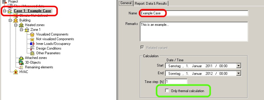
Press the “New Project” button in the Menu Bar and define a name for your project by clicking on “Case 1” in the Project Explorer. Additionally, you can enter remarks. More important is the setting of a Start and End Value as well as a suitable calculation time step like shown below in Figure 1. Furthermore, it is possible to check the entry “Only thermal calculation” (green box). Using this setting the coupled heat and moisture transport processes in the assemblies will be neglected. Only the energy transport will be considered. This will accelerate the calculation process but causes unreasonable results especially for the moisture balance as hygric interaction with assemblies is neglected. The humidity conditions inside the assemblies are not available.
STEP two : Definition of the climatic conditions
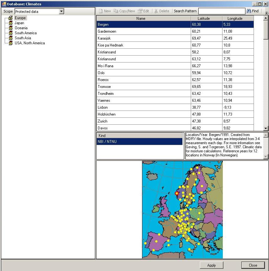
Basically, the climatic parameters, i.e. weather, influencing the simulated building can be defined here. If you want to use one of the predefined climate conditions, follow steps a) and b) shown in the picture below.

After hitting the “Browse” button another window opens (Figure 3) and the desired climate can be chosen from predefined locations by double-clicking on it.
For advanced users: It is also possible to define own climate conditions or to import own climate files.
As long as your building does not float in the air, for whatever reason, it is necessary to define at least one additional climate to give reasonable boundary conditions for the inert behavior of soil. This can be done using the “Optional Climates” tab. For the soil temperature it is accurate to select a sine curve that has its peak at about two months later than summer solstice, i.e. at the end of August / in early September in the northern hemisphere. Depending on local conditions, the amplitude of the sine curve can be modified due to the annual fluctuation of the temperature curves. This fluctuation is the difference of the mean maximum temperature of soil in warm seasons and the mean minimum temperature of soil in cold seasons. For continental climates like Siberia this amplitude may be high (high temperatures in summer, very cool winter), for maritime climate systems it is rather low. Furthermore, the mean temperature must be set. This can be approximated using the annual average air temperature. In this example we assume the climate of Holzkirchen, the WUFI®’s origin with moderate continental climate. How this can be entered in WUFI®plus can be seen in Figure 4 on the next page.
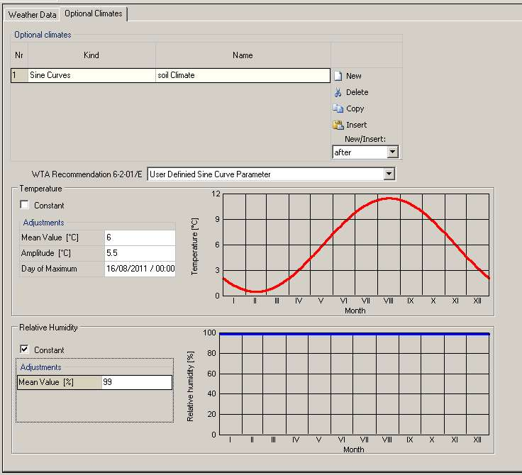
At first click at the “New” button to create a new optional climate. Then choose the sine curve and rename it to "Soil Climate" for example. In the next step choose “User Defined Sine Curve Parameter” and input following data for the temperature:
| Mean Value (°C): | 6 |
| Amplitude (°C): | 5,5 |
For relative humidity a constant mean value of 99% is adequate.
STEP three: Generate building geometry
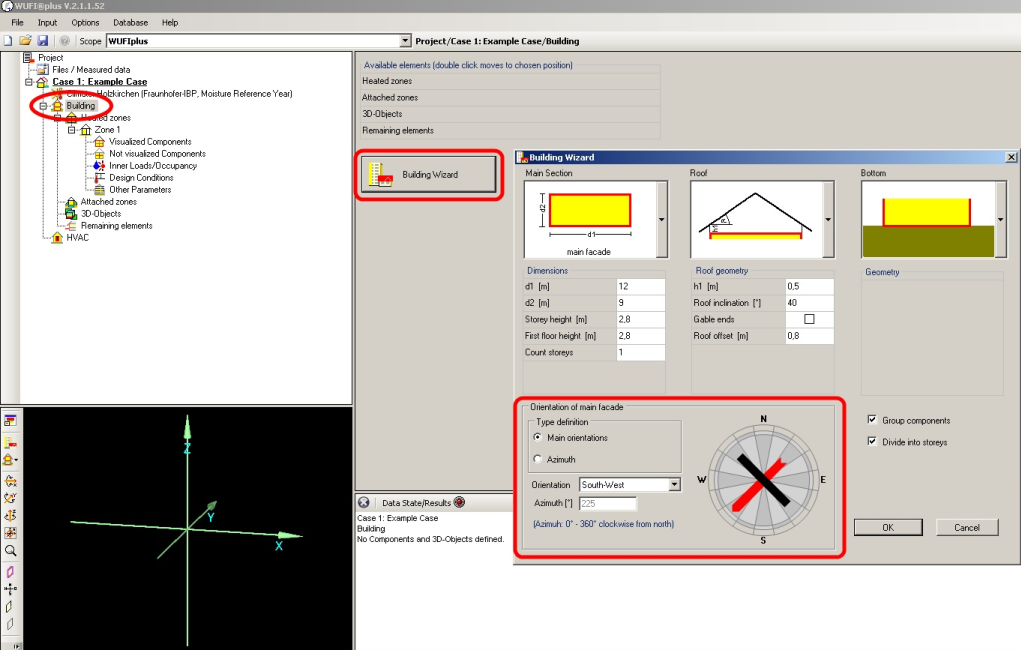
For generating the geometry, there are two basic options. Rather simple buildings or space can be created using the automatic building wizard. This tool generates a building with predefined floor plan, roof and foundation selections. Here we assume a simple case with one heated slab-on-ground zone and an inclined unheated attic. Figure 5 indicates the steps to generate a simple standalone building. There is also the possibility of defining the orientation of the main facade of the building as highlighted at the bottom of in Figure 15. If, however, a more complex building is requested, it can be created using vertices.
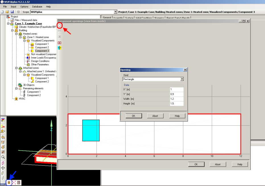
Windows are created by clicking on the desired component in the “Visualization Box” and following the blue highlighted arrow in Figure 16. The “Component Openings” window pops up. By clicking on the button highlighted by the red arrow in Figure 6, new windows can be created. In this example, one window is implemented on one outer wall (surface with normal vector in y – direction).
The X’ – axis is the orientation of the window in horizontal direction and the Y’ – axis in vertical direction. To create our window, please insert:
| X´(m) | 1 |
| Y´(m) | 0,9 |
| Width (m) | 1,2 |
| Height (m) | 1,5 |
Checking the Caption Bar of the “Component Openings” window defines whether the wall is viewed from inside or outside.
The new window will be shown under Visualized Components. So the windows and openings will appear in the navigation tree and can be edited as usual.
For advanced users: It is also possible to generate openings by using the 3D Edit tool or by defining own points.
STEP four: Definition of the components.
Primarily, a component is a surface of the building. It may be the roof, the base plate or vertical walls. As the composition of our vertical walls is mostly the same, those can be summarized as one component. This is predefined in WUFI®Plus. To change this, click on the aimed component in the Visualization Box. Afterwards, right click on this component, choose “Ungroup” and follow the instructions in accordance with your aimed modification. The “General” tab outlines basic data of a component and enables titling of components. This is especially important in case of numerous components for evaluating results.
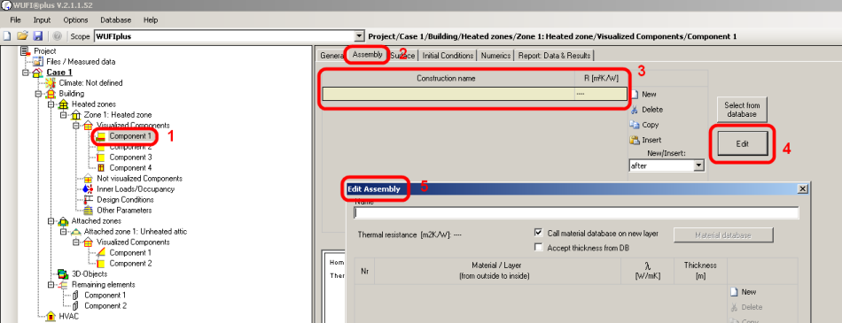
We start with Component 1 the Bottom Plate according to the steps shown in Figure 7. Choose the component you want to edit in the Project Explorer [1], next assemblies can be allocated to a component in the “Assembly” tab [2]. The Project construction list [3] shows all constructions used in a project. The highlighted one is applied to the respective component. As no constructions were assigned so far, the list is empty for one plain construction, which must be chosen. As there is no predefined geometry for the bottom plate, you have to define one, this is done by clicking the “Edit” button [4] which opens the “Edit Assembly” window [5]
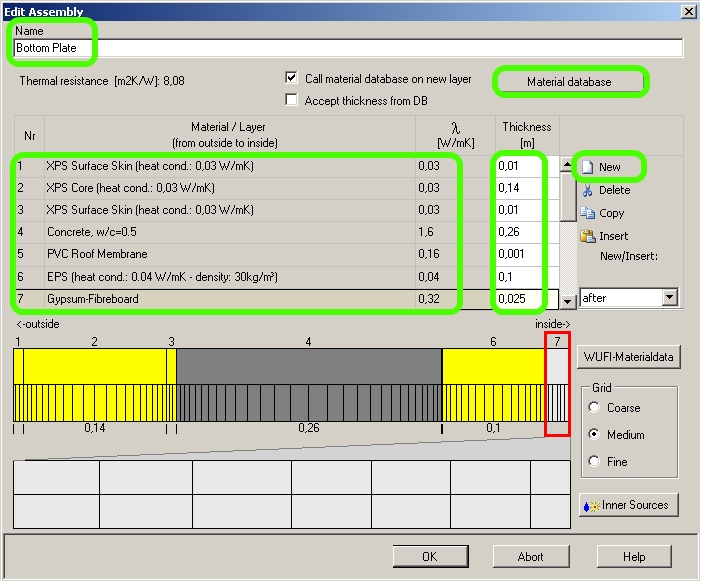
At first you have to name the Assembly. In our example it is called “Bottom Plate”. Then, by clicking on “New” you can import different layers of the construction from the database (See Figure 8). Beginning on the outside for our example the layers are:
| 1 | XPS Surface Skin (heat cond.: 0,03 W/mK) | 0,01m |
| 2 | XPS Core (heat cond.: 0,03 W/mK) | 0,14m |
| 3 | XPS Surface Skin (heat cond.: 0,03 W/mK) | 0,01m |
| 4 | Concrete, w/c=0,5 | 0,26m |
| 5 | PVC Roof Membrane | 0,001m |
| 6 | EPS (heat cond.:0,04 W/mK – density: 30kg/m³) | 0,1 |
| 7 | Gypsum Fiberboard | 0,025m |
Now you have created a new assembly called “Bottom Plate”. The bottom plate is not surrounded by air, so you have to choose the optional soil climate created in before. This works like shown in the figure below.

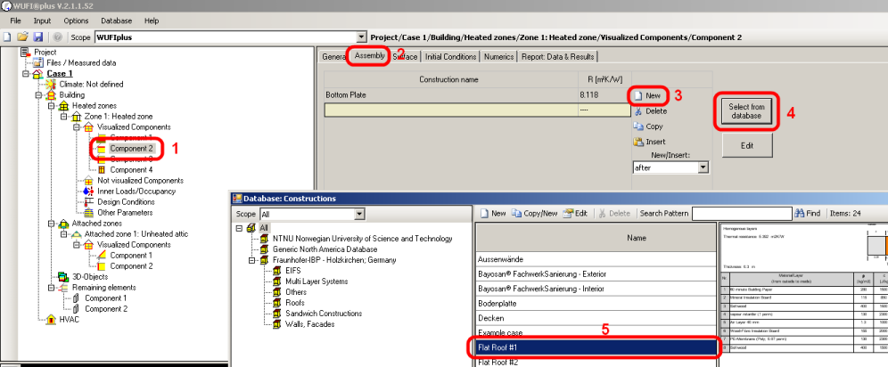
Second is Component 2, the roof, which gets an assembly assigned to it according to Figure 10. Again choose it in the Project Explorer [1], open the “Assemblies” tab [2]. Now a “New” construction needs to be added to the Construction List [3]. There is the possibility to choose predefined assemblies by clicking on “Select from database” [4]. Here Flat Roof #1 is chosen [5].
Next proceed according to the roof for Component 3, the vertical walls and choose “Lightweight timber framed wall” from the database.
Besides the “Assembly” there are various other aspects concerning the vertical walls that need to be specified.
First of all in the “Surface” section the “Thermal” subsection offers possibilities to change heat transfer resistance, absorption and emission factor according to the material of the outer surface, a general shading factor of the outer surface and solar gain. Furthermore the “Moisture” subsection allows specifying Sd-Values of the surface and inputting additional information about rain afflicting the building. There is also a “Climate on outer surface” subsection where the climatic terms of outer surface can be adjusted (see “Bottom Plate”).
Next, there is a “Initial Conditions” section where boundary conditions of the project can be altered. For example the initial relative humidity could be increased to model drying out the building.
In the “Report: Data & Results” section you could check “Retain calculation results” for hygrothermal performance assessment.
Click here for further information.
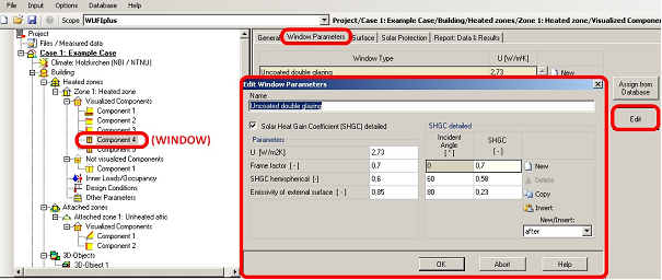
Assiging a window type to the windows from the database works similar, please choose “Uncoated double glazing” for your window.
Figure 11 illustrates the possibility of changing specific window parameters. The U parameter is the heat transfer coefficient. The frame factor enables description of opaque surfaces of the window. In effect, heat gains by solar radiation depend on the angle of incidence. In order to simulate this, the Solar Heat Gain Coefficient (SHGC) can be used. It can be set in general and with reference to the changing incident angle of solar radiation. There are appropriate predefined values, however they can be adjusted. The Emissivity of external surface is a value similar to the two previous items mentioned above. It expresses the amount of emitted radiation from the outer surface.
For advanced users: If a required material is not available in the database, it is possible to define a new material. Normally these parameters can be found in technical data sheets, necessary for this definition are:
- Bulk density [kg/m³]
- Porosity [m³/m³]
- Specific heat capacity [J/(kg K)]
- Thermal conductivity [W/ (m K)]
- Water vapor resistance factor [-]
Also user defined assemblies can be saved in the database, this is reasonable, if you want to reuse assemblies as you don’t have to define them using the “Edit” button (like you did defining the bottom plate) each time but can easily select it from the database. Watch this movie to see how user defined assemblies can be saved to the database.
STEP five: Definition of “not visualized components”
These not visualized components may be partition walls that do not separate inner climatic zones but have influence on the indoor climate as they can have heat accumulation effects due to their mass. First, a new component is established, then its surface is assigned with 25,2 m²
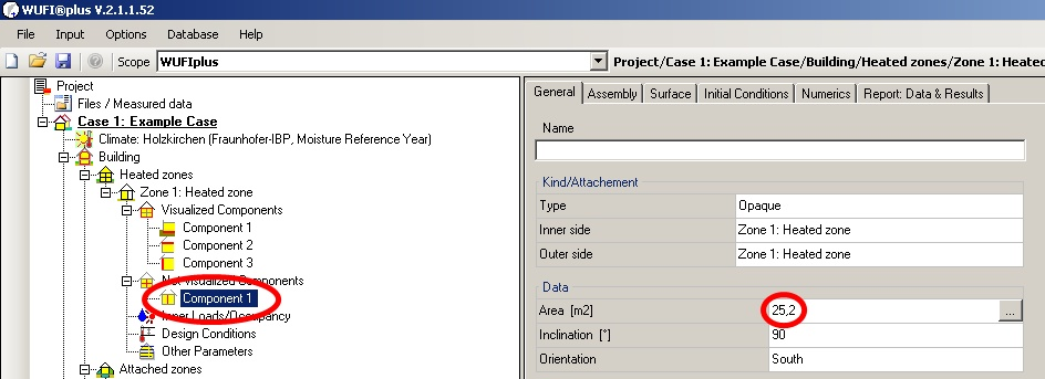
Afterward the assembly of this “Interior Wall” is defined. The proceeding is similar to the one of the bottom plate. The Layers are:
| 1 | Gypsum Board | 0,02 |
| 2 | Solid Brick ZA | 0,08 |
| 3 | Gypsum Board | 0,02 |
STEP six: Setting of inner loads (occupancy schedule)
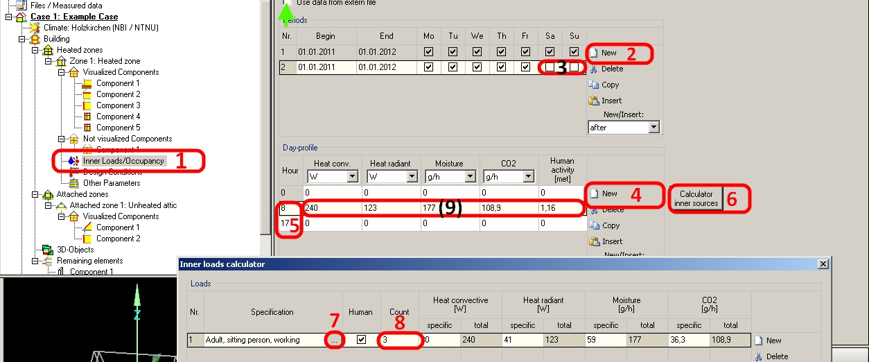
Inner loads like working people or computer produce heat, carbon dioxide and moisture. When and for how long inner loads occur is determined here. For our example, it is assumed that there are three adult people working at a desk from Monday till Friday between 8 am and 5 pm. In the following, the verification of this is explained using the steps indicated in Figure 13. Therefore, a new period must be defined and the checks for Saturday and Sunday must be removed ([2] and [3]). Note that first of all the lowest row is the primary one, and for time periods not defined by it (Saturdays and Sundays) the upper one is relevant. Afterward, the day profile for this new period must be supplemented by two entries [4]. The time is entered in 24 – hour units [5]. For our time interval beginning at 8 am, the predefined calculator is used [6] and the values for an “adult, sitting and working person” are loaded using the button “OK” [7]. The count has to be adjusted to the value three [8]. After confirming this, the numbers shown in [9] will appear on screen.
For advanced users: Another option for getting inner loads is to load an own schedule for supported file types using Files/Measured Data.
STEP seven : Defining design inner climate conditions
Step seven is related to step six. In this step you have to verify the design conditions, i.e kind of heating/cooling and the ventilation system. Preliminary it is important to know that for indoor climate conditions two basic requirements are necessary:
- a schedule to control working hours of heating, cooling, de-/humidification or ventilation system and
- a definition of capacities of these systems. see STEP eleven: Initiation of HVAC Systems or HVAC
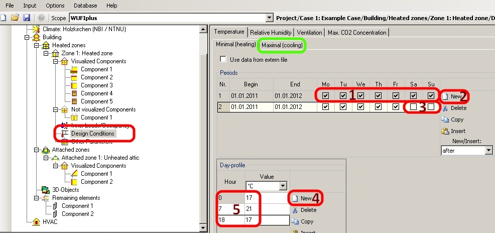
In this step, the schedules for our design conditions (the conditions to be maintained by the HVAC equipment) are defined. The indoor atmospheric conditions should conform to a certain range of temperature and relative humidity. Limits for those parameters can be set in this section. According to a healthy room temperature, in this example we use the following parameters:
| heating | |
| 0 hours | 17°C |
| 8 hours (working time) | 21°C |
| 16 hours (night) | 17°C |
| cooling | |
| 0 hours | 27°C |
| 8 hours (working time) | 24°C |
| 16 hours (night) | 27°C |
During night and on weekends, this interval can be set more widely with a range between 17 and 27 degree Celsius. For implementation in WUFI®plus follow the procedure (red numbers) depicted in Figure 14.
The next step is similar to the last one. There are three subsections in the “Ventilation” section. “Natural” means air interchange through building leaks. The leakage rate and the day profile should be inserted. During the working time the leakage rate is higher because of manual window ventilation. If there is a “Mechanical” ventilation system in the building, proceed like shown in Figure 15. At first a new schedule for working days has to be created, but note, that if a mechanical ventilation is established, do not forget to assign sufficient capacities in the HVAC menu item later on.
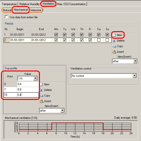
For advanced users: It is possible to consider air exchange between heated zones with different temperatures in the subsection “Interzone”. It is also possible to input values for “Relative Humidity” and “Max. CO2 Concentration”
STEP nine : Other parameters
The entries in “Other Parameters” remain unchanged in this example. The standard values in this entry are shown below.

For advanced users: The modification of solar gains can be changed in this entry, as well. In terms, the factor of direct solar radiation to the inner air and the distribution of solar radiation on the inner surfaces can be altered. The “former factor” means the fraction of solar radiation that directly heats up the inner air; the higher the value, the more direct solar heating of inner air. The latter describes different energy gains by inner surfaces. This factor can be kept proportional to the surface areas or set user-defined. Further “Other Parameters” are initial conditions of temperature, CO2 concentration and relative humidity as well as an accuracy interval of the simulation. The lower the accuracy, the faster the calculation.
STEP eight: Description of attached zones
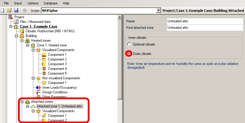
In this example, our attached zone is the roof toss. It is not heated, cooled or mechanical ventilated but normally, it also differs from the outer climate. The menu item “Attached Zones” enables the user to assign optional climates to such areas of the building. Nevertheless, in our case the outer climate is taken as reference. Otherwise it would have been necessary to define an additional optional climate.
STEP ten: 3D Objects & remaining elements
“3D objects” allows WUFI plus calculation of three dimensional thermal bridges under transient boundary conditions. In the folder “remaining Elements” surrounding of the building like trees etc. can be established.
STEP eleven: Initiation of HVAC systems
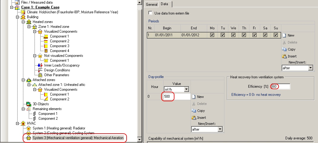
Like previously mentioned in step seven, it is important not only to schedule HVAC systems but also to assign capacities to those facilities. First it is necessary to establish these three systems like shown in Figure 18 in the red boxes. These three systems are established by hitting the “New” button three times. The type of system is selected in the “Kind” field by clicking into the blank field of the new device whereas a drop-down menu opens that suggests different system types. These are heating, cooling, de-/humidification and mechanical ventilation facilities.
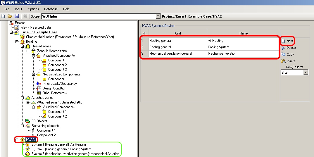
In consequence, the entries marked in the green box will appear in the project explorer. Furthermore, the facilities need characteristic values for the capacities. Please be aware that all systems are ideal systems – which means the assigned capacity is available immediately and without heat losses. Following Figure 19, the capacity of the heating system is defined 40 [kW]. In this case a schedule for the capacities is renounced as fixed facilities which serve to maintain a certain room climate are assumed. This procedure is repeated in the example for the “Cooling System”, with a capacity of 40 [kW], as well.
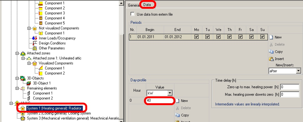
In the design conditions, the air change due to mechanical ventilation is specified with 0,8 [1/h]. In order to meet this requirement, the necessary capacity of the ventilation system must be larger than 0,8*302.4 [m³/h], due to the room volume being 9*12*2.8 [m³]. So we could set 500 m³/h for the ventilation. Also a value for heat recovery from the ventilation system thus the efficiency of the ventilation system could be set. The whole input data is:
| Heating general | 40kW |
| Cooling general | 40kW |
| Ventilation | 500 m³/h |
| Ventilation efficiency | 60% |
This issue can be seen in the red box in Figure 20. The second red box in Figure 20 indicates the possibility of simulating a heat recovery system which is common for modern ventilation systems. A reasonable value for this is 60 [%].
STEP twelve: Simulation
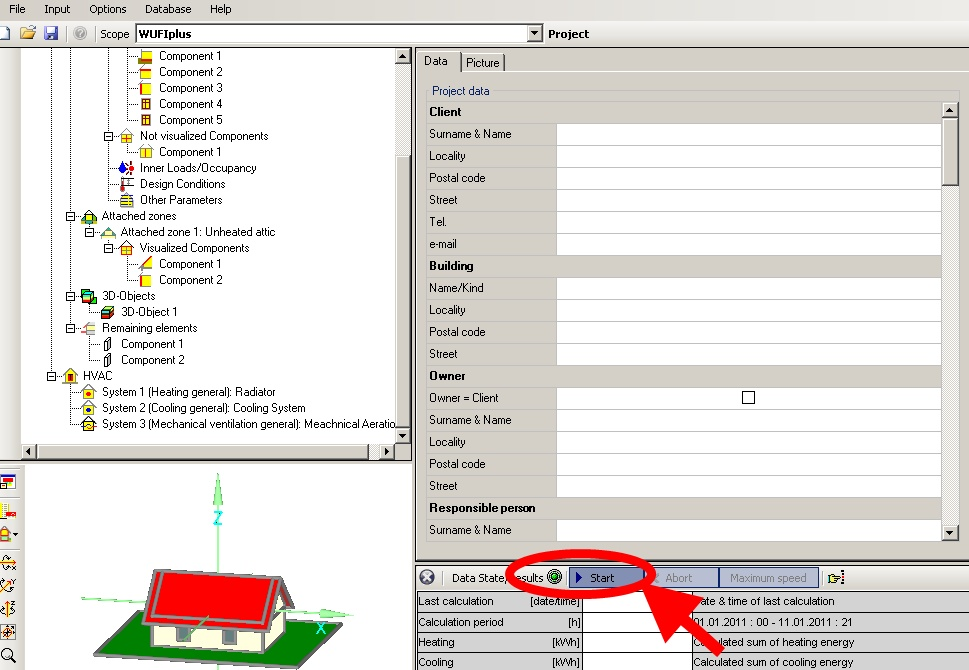
If all the above mentioned data were entered, the Status/Results Box will show the “Start” simulation button. Pressing it, hygrothermal calculation will start. If the “Start” button does not appear in the Status/Results Box and there is an error message, double-click on the error message and the program will automatically jump to the incorrect entry.
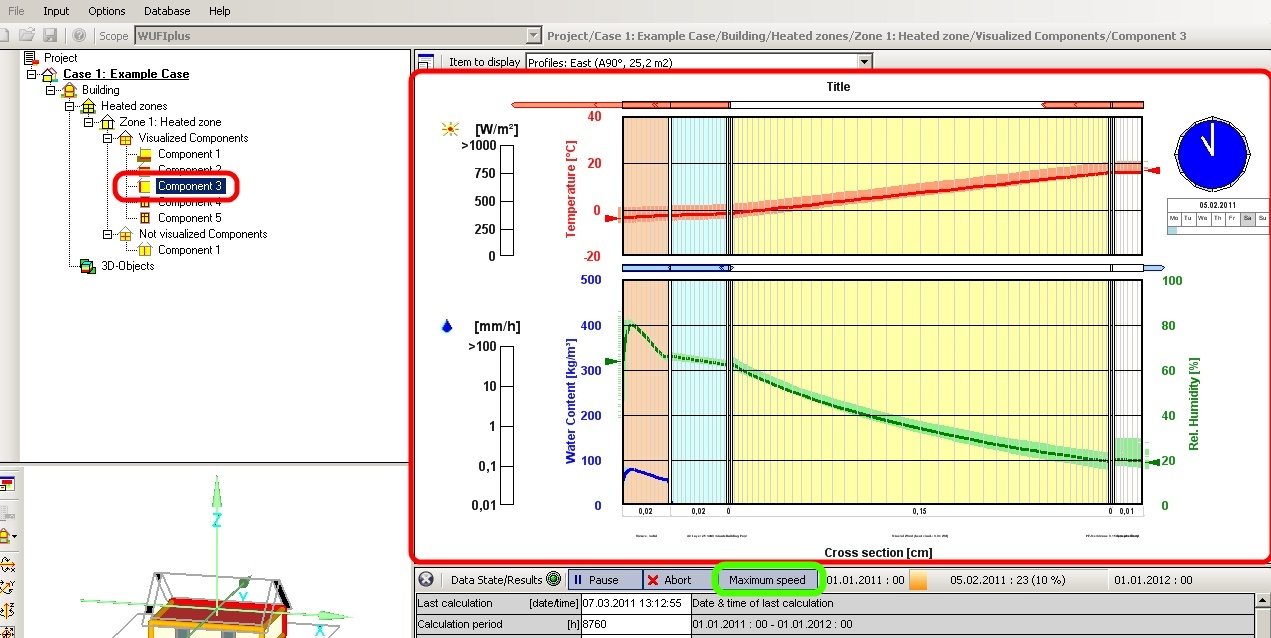
During the computation process, the simulated temperature humidity distribution in the element can be observed in real time for all components. Figure 22 shows this for our side walls. The calculation can be accelerated by deactivating this option. This can be done by clicking on the “Maximum speed” button (green box in Figure 22).
STEP thirteen: Analysis of the results
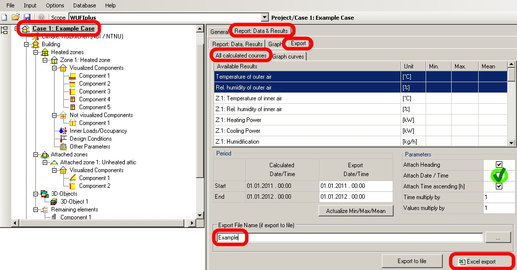
The final results of the calculations can be looked at in several ways. First, the general results can be seen like depicted in Figure 24. The Excel export, or in general, the “Export to file” button are powerful options to evaluate the calculated results as this enables the user to use external analysis programs. The export produces Excel files with values for every calculated time step. In case of not changing the calculation time step (shown in Figure 1), hourly values are written in the Excel file. It is also possible to export multiple parameters to one file by holding CTRL during clicking on the desired results. This issue is shown in Figure 24. It is also useful to export the corresponding time if you simulate over several seasons (See Figure 22 marked in green). Figure 23 illustrates the structure of an Excel Export File which had been exported according to Figure 24.
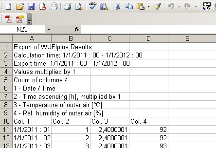
Data for the necessary energy for heating or cooling can be exported this way, as well. This may be of interest for simulating effects of insulation material. But also relative humidity, inner air temperature, components and the environment can be exported and being compared with each other. To see the whole list of possible result output parameters, scroll down the table indicated in Figure 23.
Another possibility is looking at the single building element shown in Figure 25. If desired, the box “Retain calculation results” needs to be checked. This box is highlighted in Figure 25 with green color.
